Modelling overlapping slabs with variable loads in ETABS

It’s very common, in the course of designing concrete structures, that you will have to model slabs and their loads for purposes such as mass estimation and load calculation. And when dealing with complicated slabs that have variable thickness and loading, you may end up with many overlapping elements, which obscures the load calculation. It may be hard to reason about how the load is being applied if you do not understand how ETABS treats overlapping areas.

Computers and Structures Inc. have a short comparison of how SAFE and ETABS determine the applicable load and stiffness properties to use at any given location on the slab. Unfortuneately, the behavior isn’t consistant between these two programs, as explained below.

Load Rules

In ETABS, the slab with smallest area takes precedence. The exception to this rule is Null shells, which will superimpose their loads onto the larger slab.

In SAFE, the slab loadings always add together.

In both programs, it is recommended to draw a single large area with one area and loading, and then draw overlapping smaller areas to change the loading and/or thickness. This tends to reduce the number of automatic meshing errors (such as adjacent elements not sharing the auto-generated mesh nodes, and hence not being connected along an edge)

Comparison Models

To compare and verify the slab loading behavior in ETABS, I present a very simple model.

In this model, there is a 10ft x 10ft slab area supported by a column in each corner. A 5ft x 10ft area is overlapped on this area, with variable loads and properties. We will neglect the self weight of the structure, and only look at assigned live loads.

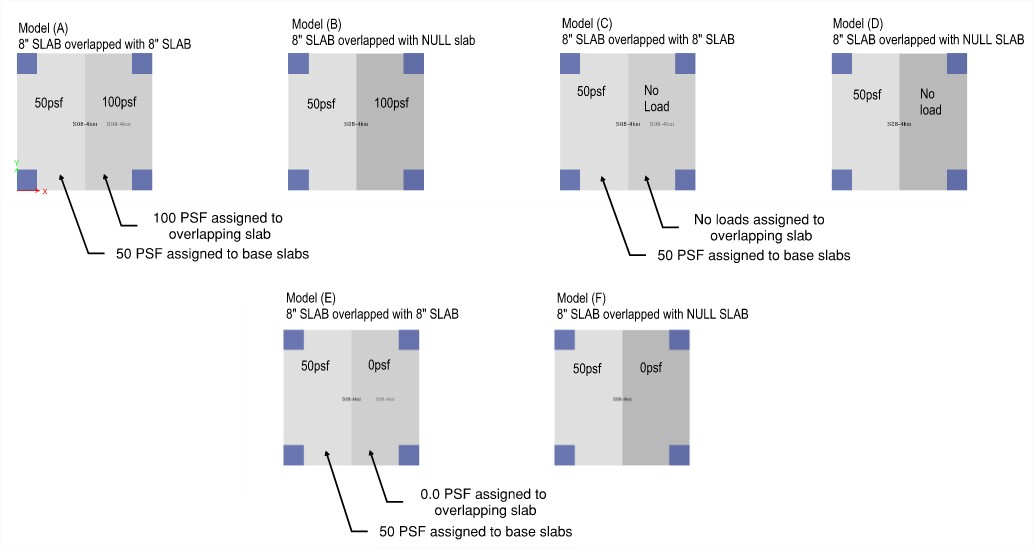
Models A, C, and E all contain an 8” base slab and an overlapping 8” slab. The base slab is assigned 50psf live load, and the overlapping slab is assigned 100psf, No load, and 0psf load for each model, respectively.

Models B, D, and F all contain an 8” base slab and an overlapping Null slab. The base slab is assigned 50psf live load, and the overlapping slab is assigned 100psf, No load, and 0psf load for each model, respectively.

Results

The total base reaction in the vertical direction are summarized below for each model.

First, lets get accustomed to the numbers. The basic 10ft x 10ft slab is loaded with: $$P_1 = (50 \mathrm{ psf})(10 \mathrm{ft})(10 \mathrm{ft})/1000 = 5.0 \mathrm{kip}$$

The overlapping 5ft x 10ft slab is loaded with either 100psf (Model A, B), no load assigned (Model C, D), or 0psf assigned (Model E, F): $$P_2 = (100 \mathrm{ psf})(5 \mathrm{ft})(10 \mathrm{ft})/1000 = 5.0 \mathrm{kip} \textrm{ (or 0 kip)}$$

But these two pieces aren’t necessarily added together. We need to follow the ETABS load rules.

In Model A the load rules state that since each slab is assigned a property, the smaller slab load will govern over its defined area. Hence the load calculation for the structure becomes: $$P_{A} = (50 \mathrm{ psf})(5 \mathrm{ft})(10 \mathrm{ft})/1000 + (100 \mathrm{ psf})(5 \mathrm{ft})(10 \mathrm{ft})/1000$$ $$P_{A} = 2.5 + 5.0 = 7.5 \mathrm{kip}$$

In Model B, the load rules state that the Null shell will superimpose the load on top of the basic slab, such that the net load in the overlap is 150psf. Hence the load calculation for the structure becomes: $$P_{B} = (50 \mathrm{ psf})(10 \mathrm{ft})(10 \mathrm{ft})/1000 + (100 \mathrm{ psf})(5 \mathrm{ft})(10 \mathrm{ft})/1000$$ $$P_{B} = 5.0 + 5.0 = 10.0 \mathrm{kip}$$

In Model C and E the load rules state that since each slab is assigned a property, the smaller slab load will govern over its defined area. This applies regardless of whether the slab is defined with 0psf or no loads at all. Hence the load calculation for the structure becomes: $$P_{C} = P_{E} = (50 \mathrm{ psf})(5 \mathrm{ft})(10 \mathrm{ft})/1000 + (0.0 \mathrm{ psf})(5 \mathrm{ft})(10 \mathrm{ft})/1000$$ $$P_{C} = P_{E} = 2.5 + 0.0 = 2.5 \mathrm{kip}$$

In Model D and F, the load rules state that the Null shell will superimpose the load on top of the basic slab, and this behavior doesn’t change regardless of whether the Null shell is assigned 0psf or no loads at all. Hence the load calculation for the structure becomes: $$P_{D} = P_{F} = (50 \mathrm{ psf})(10 \mathrm{ft})(10 \mathrm{ft})/1000 + (0 \mathrm{ psf})(5 \mathrm{ft})(10 \mathrm{ft})/1000$$ $$P_{D} = P_{F} = 5.0 + 0 = 5.0 \mathrm{kip}$$

Recommendation for complex slabs

It’s easy to mix up the load calculation behavior in a complicated slab with variable thicknesses and loads. I always recommend following the approach of Model (A):

• Give every slab a property - do not use null areas.
• Draw smaller areas to specify the total load desired at any given location.
• The loading at any location will be equal to the loading assigned to the smallest slab that exists at that location.

Its also prudent to verify loads using some simple hand checks, especially if you are unsure of the behavior.